Regression and line fit
We use these two terms much more than we think. We try to predict or find out if two variables are related to each other, or if we can explain one through the other.
- Finding if two variables have a relation between them (whatever it is), is what we call correlation.
- Trying to explain one of them, from the other, is what we know as regression.
Before starting the study of these techniques, we must explain what is a dependent and independent variable. We will see it with two examples.
- The number of piglets weaned per sow and year is a function of the fertility of the farm, then fertility is the independent variable, and the number of piglets is the dependent variable (it depends on fertility).
- The number of weaned piglets per sow and year is a function of perinatal mortality. Therefore, perinatal mortality is the independent variable and the number of piglets the dependent variable (it depends on perinatal mortality).
But neither perinatal mortality is a function of fertility, nor vice versa, although they may be related (for example, if an infectious process affects the farm).
We should not these terms with causality. The fact that there is a correlation, or that we carry out a regression analysis between the variables, does not mean that there is a cause-effect or causality relation between these two variables. We must establish this cause-effect relation with biological, technical, bibliographic criteria …
In this article, we explain regression in detail and develop a case study to make it easier to understand. As usual, with common variables in the Animal Production industry. If you want to read more what is the correlation, and a practical case, we have it published in this article.
Regression
Regression has two forms, the descriptive (we see what “there is”) and the inferential (we draw conclusions).
- The descriptive one studies the linear relation between two variables establishing the equation of the line (from now on we will call it the regression line) that best fits these data and decomposing the total variability of the dependent variable in two parts: the part of the total variability explained by the regression line from the independent variable and the unexplained part (also called residual), and which helps us to evaluate the fit of the line. We will see how to explain the total variability in this way.
- The inferential one assumes that the study data is from a random sample. Then, we evaluate whether the variables are related to the population. If so, we can estimate which regression predicts best the relation between the dependent and the independent variable.
Regression line
We have tried to avoid mathematical explanations. However, in regression, it is essential to understand the mathematical logic, since through its knowledge we will be able to perfectly understand the study of linear regression, which will help us to explain later the general linear model that is used for most experiments in health sciences.
Firstly, we are going to explain how, through a series of data, we obtain a fit line, the regression line. To do this, we shall remember the equation of the line and the meaning of its coefficients. The equation of a line is given by the formula: y = a + bx, where a and b are the coefficients of the line:
- a indicates the value for the point x = 0, which is the intersection point of the line with the ordinate axis (y-axis). If we take x = 0, then bx = 0 and y = a;
- b indicates the slope of the line, that is, the increase in y for each unit that x increases. If we take a = 0 and x = 1, then y = b. y where x and y are the values of the variables:
- y is the value for the dependent variable, that is, the explained.
- x is the value for the independent variable, that is, the one that explains.
If we see it graphically, it is very easy to understand (figure 1).

The value a = 1 indicates the intersection point of the line with the ordinate axis and the value b = 1.5 indicates the increase of the variable y for each unit that the variable x increases. The regression line is therefore y = a + bx = 1 + 1.5x.
Fit criterion of the regression line
And how to fit a line to a point cloud? What criteria should we follow? We will see it with the minimum mathematical expressions and with a series of graphs.
Imagine the graph in Figure 2.

If we draw a line to describe these three points, we could say that the line that appears would describe the three points quite well, at least from a visual point of view. Due to the variability of the data, if this line is used to predict the yi value of a subject i based on its xi value, it is observed that there is a difference ei called residual, which represents the prediction error:
ei = yi – yi.
The criterion of the fit line should minimize the set of residuals ei. One might think of minimizing the sum of the absolute value of the residuals, but this condition leads to a very unsatisfactory fit. The generally adopted solution is to minimize the sum of the squared residuals because this criterion has an easy mathematical solution and produces correct fits in most situations.
Let’s see it in an empirical way.
In the following image, we have a graph with the same points as in figure 2, but with two different adjustment lines.

The equations of these two lines are:
Purple line: y = 0.5x
Green line: y = 2 + 0.5x
Which of the two lines best explains the relation between x and y? We have talked about three criteria, so now we are going to see which line would be chosen in each case and which of the two lines (and with what criteria) we take:
■ If we follow an “intuitive” criterion, we can choose when answering the question, which one fits the best visually?
■ If we follow the criterion, what is the sum of the absolute values of the residuals in each of the two lines worth? We must do these sums:
- Purple line: ei = 0 + 2 + 0 = 2
- Green line: ei = 1 + 1 + 1 = 3
■ Finally, if we follow this criterion: how much is the sum of the squared residuals of each line?
- Purple line: ei = 02 + 22 + 02 = 4
- Green line: ei = 12 + 12 + 12 = 3
Choosing the line
You will observe that the purple line has two null residuals and a residual equal to 2, while the green line has all its residuals equal to 1. In absolute value, the sum of residuals is greater in the green line than in the purple one, but when we square the residuals, the sum is less on the green line than on the purple line.
The reason for squaring the residuals is because large differences are magnified, and the least-squares fit looks for a compromise line that avoids very large residuals. This property has the consequence that the mathematically estimated line tends to coincide with the one that the human eye would adjust. We are left with the least-squares criterion (the third criteria).
An example with Síagro
Now that we have seen the mathematical method, we are going to see how to carry out the regression with Síagro with the following data:
| piglet | ADC | ADG |
| 1 | 1.064 | 532 |
| 2 | 1.168 | 556 |
| 3 | 905 | 411 |
| 4 | 1.124 | 562 |
| 5 | 1.100 | 523 |
| 6 | 1.198 | 544 |
| 7 | 935 | 467 |
| 8 | 1.088 | 518 |
| 9 | 1.109 | 554 |
| 10 | 1.009 | 438 |
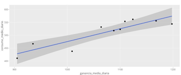
To study the regression between the Average Daily Gain (ADG), the dependent variable, and the Average Daily Consumption (ADC), the independent variable, we only have to access to Prediction Models / Linear from the control panel and select our variables. It’s that simple, and the application will return the following output:
| term | estimate | std.error | statistic | p.value | Sig | ||||||||||||
| (Intercept) | -23,0443 | 97.7 | -0.236 | 0.819 | |||||||||||||
| CMD | 0.4986 | 0.091 | 5.48 | 0.000588 | *** | ||||||||||||
| r.squared | adj.r.squared | sigma | statistic | p.value | df | logLik | AIC | BIC | deviance | df.residual | nobs | ||||||
| 0.79 | 0.763 | 25.9 | 30 | 0.000588 | 1 | -45.6 | 97.2 | 98.1 | 5.36e+03 | 8 | 10 | ||||||
We are only going to explain some of the data that appears in this output, leaving a broad explanation for the next article (but do not hesitate to contact our team if you have further doubts). What would be the equation of the regression line? Just recall that in our case the variable y is y = ADG and the variable x is x = ADC.
ADG = -23.0443 + 0.4986 ADC
That is, the estimated coefficients of a and b are what Síagro (and R) calls Estimate. From the above equation we can say that for each unit of ADC, the ADG increases 0.4986.
But … can we really trust that relation? Or in another way: is the coefficient b different from 0?
This question involves going from description to inference, as we said at the beginning of the article. This is answered with a t-test with null hypothesis b = 0 and alternative b ≠ 0. In this case, the p-value is less than 0, 05 (p-value: 0.000588) and therefore we reject the null hypothesis, that is, b is different from 0.
We can also say that the CMD explains 78.96% of the GMD.
We will see in the next article further explanations of variability. We recommend you to be subscribed to our newsletter if you do not want to miss it!!