How do we determine the effect on the average gain of piglets if we include fishmeal in their diet and in different amounts?
A statistical study often compares more than two populations. Therefore, Statistics includes specific methods to compare any number of means and be useful in any context. To clarify, let’s see an example of a comparison of two means and another of multiple comparisons:
- Comparison of two means: Evaluate the effect of including fishmeal in the diet of piglets on their average daily gain. In this case, we evaluate the effect of one variable on the mean of another variable.
- Multiple comparisons: Evaluate the effect of including fishmeal in the diet of piglets in different amounts on their average daily gain.
In this post, we are going to solve the title question that responds to a case of multiple comparisons: What analysis do we use to determine the effect that it has, on the average daily gain (GMD, from now on) of the piglets, to include in the diet fish meal in different amounts?
Let’s start!
Suppose that three diets have been distributed to 20 piglets in the prestarter stage:
- Diet 1 contained 0% fishmeal.
- Diet 2 contained 4% fishmeal.
- Lastly, diet 3 contained 8% fishmeal.
The results obtained in terms of average daily gain were as follows:
| ADG Diet 0% (H0) | A.D.G. Diet 4% (H4) | A.D.G. Diet 8% (H8) |
| 0,224 | 0,248 | 0,265 |
| 0,211 | 0,240 | 0,187 |
| 0,227 | 0,228 | 0,289 |
| 0,228 | 0,266 | 0,250 |
| . | . | . |
| . | . | . |
| . | . | . |
| 0,250 | 0,210 | 0,268 |
| 0,235 | 0,265 | 0,221 |
Table 1: Average daily gain (ADG) of piglets according to the amount of fishmeal included in the diet.
First, we are going to explore our data and extract some basic statistics (for this exercise, we are going to use the Síagro statistical program).
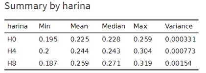
Table 2: Exploratory Analysis
As we can see, the GMD increases as the fishmeal content of the piglets’ diet also increase: the mean GMD for the diet with 0% fishmeal is 0.224, for the diet of 4% is 0.244, and that for the 8% diet is 0.259. Now, the question we should ask ourselves is the following: are these differences statistically significant?
The problem of multiple comparisons
First, let’s start by naming the GMD averages. For the diet with 0% fishmeal, the mean will be m1, for the diet with 4% fishmeal we will call it m2, and for the diet with 8% fishmeal, the mean will be m3.
If we intended to compare these three means, we could use the two-sample t-test several times, but this is a waste of time since we have specific statistical models for this context.
The problem of comparing several means together can be solved by an Analysis of Variance or ANOVA.
Its difficulty is minimal, although greater than in the case of significance tests. As we will see, these tests allow us to compare all the means together and to discern if there are significant differences among them. Once we detect the differences, and in a subsequent analysis, we will be able to determine the differences between each of the means separately.
Factorial Analysis of Variance. Analysis of variance F test
A singularity of statistics is that one of the methods to compare means is called Analysis of Variance (ANOVA, hereinafter). The reason is that this test is carried out by comparing two types of variation. ANOVA is a general method for studying sources of variation in responses. The comparison of several means is called factorial Analysis of Variance. It is a factor because the response variable (in our example, GMD of the piglets), is only influenced by another variable (in our example, the content of fishmeal in the diet). The test of Analysis of Variance to compare various means is called the F test.
The F statistic used to compare various means has the following form:
F = variation among sample means/variation among individuals of the same sample
The F statistic only takes positive or zero values. It will be zero when the means are all equal. In fact, the effect of chance creates some differences between the sample means, even when the population means are the same. Thus, when the null hypothesis is true, we expect F to take values close to one. As the sample means are further apart, the value of F becomes larger.
The large values of F constitute a reliable test against the null hypothesis, leaving us thinking that the correct hypothesis is the alternative, the one that contemplates that some of the sample means are not equal to the others.
There is no better explanation than what can be seen in an example.
In this way, let’s follow the thread of the example we raised in the introduction. We want to test the null hypothesis that there are no differences among the GMD of the piglets for the three diets with different fishmeal content. That is to say:
- H0: m1 = m2 = m3
The alternative hypothesis states that there is a difference among the means, that is, not all means are the same:
- Ha: m1 ¹ m2 ¹ m3
The Ha considers the case that m1 = m2, but that m3 has a different value, or any other combination. The contrast of H0 against Ha is called the ANOVA F test.
ANOVA in Síagro
To continue with the ANOVA of the example we are going to use the Síagro program. Once the recorded data has been entered, we will go to the Prediction Models option, which will always be by default in the control panel, and then, to ANOVA.

Image 1. Access to ANOVA in Síagro.
Next, we select the variable GMD and the factor flour. In the first, we have the data collected in the field and, in the second, the three factors: H0, H4, and H8.
The result is the following:

Where:
- Df: degrees of freedom
- Sumsq: sum of squares
- Means: Average of squares
- Statistic: Contrast statistic F
- P-value: Probability
And,
- Harina (flour): Among groups
- Residuals: Within groups.
Let’s look at the test statistic F, F = 6.81. As we said, a higher value of F gives us an idea that the null hypothesis is not correct. Now let’s look at its probability (p-value), which is 0.00223. If the probability value is below 0.05 (the traditionally accepted level of significance), we can affirm that there is evidence that the three types of diet are not the same, or that one of them is different from the others. That is, they affect in a different way the Average daily gain of the piglets. We are in a position to reject the hypothesis and accept the alternative hypothesis as certain.
Multi-factorial Analysis of Variance
In the example, the factor that could disturb our response variable, Average Daily Gain, was only the fishmeal content of the diet. This is the simplest case that we can find when we analyze some data and want to compare means. Let’s suppose another situation …
What would have happened if we had separated the piglets into two halves and supplied them with two different diets for energy, apart from the fishmeal content?
The variable Average Daily Gain would not only be influenced by the fish meal factor, but it would also be (or could be) influenced by the amount of energy provided by the diet. In fact, the number of factors to include in an analysis can be very broad, but then the analysis would be overly complicated.

